Model: GraniteMoeHybridMambaLayer on Nvidia H200

Summary

Using our agentic AI compiler (yasp.compile), we achieved a 6.25x speedup on the Mamba hybrid block of IBM's Granite 4.0. The dominant optimization was an algebraic rewrite: yasp.compile identified that a memory-bound element-wise multiply followed by a reduction was algebraically equivalent to a batched matrix multiplication (bmm), and substituted accordingly. In this specific instance, the switch of operations eliminated a ~48 GB intermediate tensor and the memory transfers it caused, which dominated the original layer's runtime. How this layer speedup translated to a full model speedup is detailed in this post.

Yasp's Agentic AI Compiler: yasp.compile

Writing fast GPU kernels is hard and time-consuming. The gap between generic, poorly optimized code and what the hardware is actually capable of can be enormous. Closing this gap traditionally requires scarce, expensive expertise and significant engineering time. yasp.compile closes the gap without manual kernel tuning: an agentic system that analyzes a machine learning model and generates optimized, hardware-specific code automatically. It operates at any granularity: a single operation, a full layer, or an entire model, and produces kernels tuned to your specific hardware, for both inference and training. The case study below demonstrates this on the Mamba-2 block of IBM's Granite 4.0 architecture.

The Bottleneck: A 48 GB Intermediate Tensor

The reference PyTorch implementation computes an element-wise multiply between two 6D tensors followed by a sum reduction over the last dimension. The pseudo-code below illustrates the pattern. input1 [32, 1, 256, 1, 48, 128] and input2 [32, 1, 1, 256, 48, 128] are each ~192 MB. Broadcasting across their mismatched size-1 dimensions, the resulting tensor inter expands to [32, 1, 256, 256, 48, 128]; ~12.9 billion float32 values (~48 GB); which is materialized in GPU memory only to be immediately discarded after the reduction.

# Reference code, variables renamed for readability
# input tensor sizes:
# input1 [32, 1, 256, 1, 48, 128]
# input2 [32, 1, 1, 256, 48, 128]

inter:            "f32[32, 1, 256, 256, 48, 128]" = torch.ops.aten.mul.Tensor(input1, input2)
reduction_result: "f32[32, 1, 256, 256, 48]"      = torch.ops.aten.sum.dim_IntList(inter, [-1])
inter = None

# Reference code, variables renamed for readability
# input tensor sizes:
# input1 [32, 1, 256, 1, 48, 128]
# input2 [32, 1, 1, 256, 48, 128]

inter:            "f32[32, 1, 256, 256, 48, 128]" = torch.ops.aten.mul.Tensor(input1, input2)
reduction_result: "f32[32, 1, 256, 256, 48]"      = torch.ops.aten.sum.dim_IntList(inter, [-1])
inter = None

# Reference code, variables renamed for readability
# input tensor sizes:
# input1 [32, 1, 256, 1, 48, 128]
# input2 [32, 1, 1, 256, 48, 128]

inter:            "f32[32, 1, 256, 256, 48, 128]" = torch.ops.aten.mul.Tensor(input1, input2)
reduction_result: "f32[32, 1, 256, 256, 48]"      = torch.ops.aten.sum.dim_IntList(inter, [-1])
inter = None

This operation is memory-bound: the GPU spends more time transferring data than computing. PyTorch Inductor (PyTorch's default compiler backend) cannot resolve this; it materializes the full ~48 GB intermediate tensor and generates a Triton kernel for the multiply-reduce, as shown below.

# snippet
@triton.jit
def triton_red_fused_mul_sum_7(in_ptr0, in_ptr1, out_ptr0, xnumel, r0_numel, XBLOCK : tl.constexpr, R0_BLOCK : tl.constexpr):
    xnumel    = 100663296
    r0_numel = 128

    # ... cut here for brevity

    # 'xnumel'   = 100,663,296 is the number of output elements (32 * 256 * 256 * 48)
    # 'r0_numel' = 128 is the reduction size per output element
    # In combination this results in 100M * 128 = 12.9B input elements total.
...

# snippet
@triton.jit
def triton_red_fused_mul_sum_7(in_ptr0, in_ptr1, out_ptr0, xnumel, r0_numel, XBLOCK : tl.constexpr, R0_BLOCK : tl.constexpr):
    xnumel    = 100663296
    r0_numel = 128

    # ... cut here for brevity

    # 'xnumel'   = 100,663,296 is the number of output elements (32 * 256 * 256 * 48)
    # 'r0_numel' = 128 is the reduction size per output element
    # In combination this results in 100M * 128 = 12.9B input elements total.
...

# snippet
@triton.jit
def triton_red_fused_mul_sum_7(in_ptr0, in_ptr1, out_ptr0, xnumel, r0_numel, XBLOCK : tl.constexpr, R0_BLOCK : tl.constexpr):
    xnumel    = 100663296
    r0_numel = 128

    # ... cut here for brevity

    # 'xnumel'   = 100,663,296 is the number of output elements (32 * 256 * 256 * 48)
    # 'r0_numel' = 128 is the reduction size per output element
    # In combination this results in 100M * 128 = 12.9B input elements total.
...

The Fix: Recognize the Hidden Matrix Multiply

The element-wise multiply followed by a sum over the last dimension in this operation is mathematically equivalent to a batched dot product (i.e., a matrix multiplication). For two tensors A[b_1, ..., b_n, i, d] and B[b1, ..., b_n, j, d], the pattern:

is exactly C = A @ B^T, a standard GEMM. yasp.compile recognized this pattern and rewrote the operation as:

# Optimized: batched matrix multiply and preparing the tensors
# Variables renamed for clarity
# input1 [32, 1, 256, 1, 48, 128]
# input2 [32, 1, 1, 256, 48, 128]
in_perm1: "f32[32, 1, 256, 48, 128]" = torch.ops.aten.view.default(input1, [32, -1, 256, 48, 128])
in_perm2: "f32[32, 1, 256, 48, 128]" = torch.ops.aten.view.default(input2, [32, -1, 256, 48, 128])

in_bmm1: "f32[1536, 256, 128]" = in_perm1.permute(0, 1, 3, 2, 4).contiguous().reshape(32 * 48, 256, 128)
in_bmm2: "f32[1536, 256, 128]" = in_perm2.permute(0, 1, 3, 2, 4).contiguous().reshape(32 * 48, 256, 128)

inter_bmm:        "f32[1536, 256, 256]"      = torch.bmm(in_bmm1, in_bmm2.transpose(-1, -2))
reduction_result: "f32[32, 1, 256, 256, 48]" = inter_bmm.reshape(32, 48, 256, 256).permute(0, 2, 3, 1).unsqueeze(1).contiguous()

# Optimized: batched matrix multiply and preparing the tensors
# Variables renamed for clarity
# input1 [32, 1, 256, 1, 48, 128]
# input2 [32, 1, 1, 256, 48, 128]
in_perm1: "f32[32, 1, 256, 48, 128]" = torch.ops.aten.view.default(input1, [32, -1, 256, 48, 128])
in_perm2: "f32[32, 1, 256, 48, 128]" = torch.ops.aten.view.default(input2, [32, -1, 256, 48, 128])

in_bmm1: "f32[1536, 256, 128]" = in_perm1.permute(0, 1, 3, 2, 4).contiguous().reshape(32 * 48, 256, 128)
in_bmm2: "f32[1536, 256, 128]" = in_perm2.permute(0, 1, 3, 2, 4).contiguous().reshape(32 * 48, 256, 128)

inter_bmm:        "f32[1536, 256, 256]"      = torch.bmm(in_bmm1, in_bmm2.transpose(-1, -2))
reduction_result: "f32[32, 1, 256, 256, 48]" = inter_bmm.reshape(32, 48, 256, 256).permute(0, 2, 3, 1).unsqueeze(1).contiguous()

# Optimized: batched matrix multiply and preparing the tensors
# Variables renamed for clarity
# input1 [32, 1, 256, 1, 48, 128]
# input2 [32, 1, 1, 256, 48, 128]
in_perm1: "f32[32, 1, 256, 48, 128]" = torch.ops.aten.view.default(input1, [32, -1, 256, 48, 128])
in_perm2: "f32[32, 1, 256, 48, 128]" = torch.ops.aten.view.default(input2, [32, -1, 256, 48, 128])

in_bmm1: "f32[1536, 256, 128]" = in_perm1.permute(0, 1, 3, 2, 4).contiguous().reshape(32 * 48, 256, 128)
in_bmm2: "f32[1536, 256, 128]" = in_perm2.permute(0, 1, 3, 2, 4).contiguous().reshape(32 * 48, 256, 128)

inter_bmm:        "f32[1536, 256, 256]"      = torch.bmm(in_bmm1, in_bmm2.transpose(-1, -2))
reduction_result: "f32[32, 1, 256, 256, 48]" = inter_bmm.reshape(32, 48, 256, 256).permute(0, 2, 3, 1).unsqueeze(1).contiguous()

The 48 GB intermediate tensor is never materialized. The sum reduction is now the inner loop of the GEMM, and cuBLAS handles the computation with highly optimized algorithms.

Why This Matters: From Memory-Bound to Compute-Bound

This rewrite fundamentally changed the character of the workload, not just its memory footprint. On a GPU, the scheduler dispatches thread blocks (groups of threads, here 128 per block) to compute cores. Launching millions of thread blocks burns cycles on scheduling and address arithmetic rather than computation.

The 1024x reduction in thread blocks directly cuts that overhead. In addition, there is a shift in the most utilized pipeline: the ALU (execution of integer and logic instructions) pipeline handles integer arithmetic and address calculations; the FMA (Fused Multiply-Add) pipeline executes floating-point math. Nsight Compute profiling (Figs. 1–2) shows the GPU moving from ALU-dominated to FMA-dominated execution, confirming cycles are now spent on computation. Arithmetic intensity increased, and so did effective FLOP/s, translating directly into the 6.25x layer speedup. The layer speedup is below the isolated kernel speedup (~34x) because the full layer contains additional operations beyond this kernel.

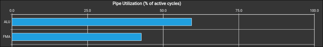
Figure 1: Pipeline utilization of the PyTorch Inductor solution

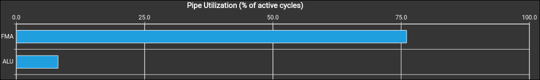
Figure 2: Pipeline utilization of the yasp.compile solution

The Nsight Systems trace in Fig. 3 shows the Inductor baseline: the Triton reduction kernels dominate the timeline, confirming the memory-bound reduction was the primary bottleneck.

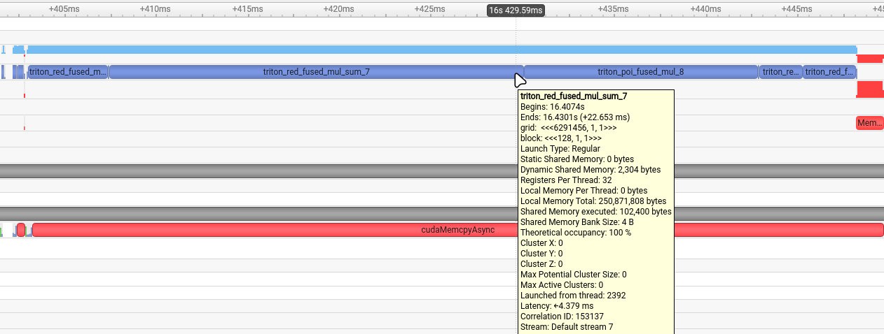
Figure 3: Nsight Systems timeline of the Inductor generated multiply and reduction kernel.

In the yasp.compile trace (Fig. 4), cuBLAS GEMM calls replace the reduction kernels entirely, executing ~34x faster and cutting the overall layer runtime.

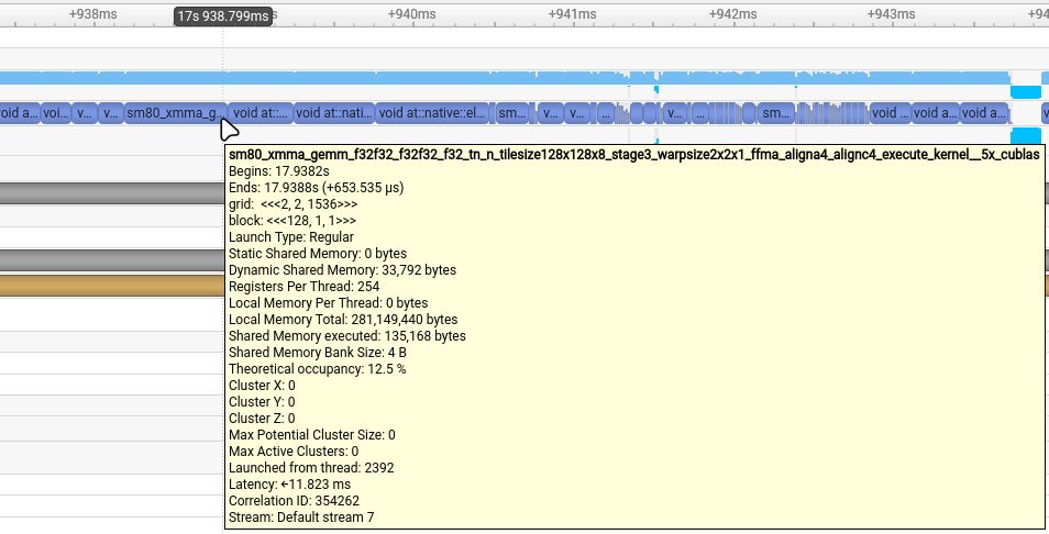
Figure 4: Nsight Systems timeline of the yasp.compile used GEMM kernel.

Beyond the Core Optimization

The same einsum-to-bmm pattern appeared in four places total within the Mamba layer. We focused on the instance with the largest intermediate tensor here.

In addition, yasp.compile fused several element-wise operation chains into custom Triton kernels:

• Fused SiLU: x ‧ sigmoid(x) in a single pass

• Fused RMS Norm: Combines square, mean, rsqrt, and scale into a single kernel with float32 accumulation

• Fused softplus + clamp: Merges an add, log(1 + exp(x)), and clamp into one kernel with numerically stable branching

• Fused SiLU-gate multiply: Combines x ‧ silu(gate) into a single kernel, avoiding an intermediate tensor

While these Triton fusions can contribute to the overall speedup, the four bmm rewrites account for the majority of the performance gain.

Correctness

Performance gains are meaningless without correctness. All tensors returned by the optimized layer match the results of the Inductor reference within tight tolerances (verified via torch.allclose with atol=1e-3 and rtol=1e-8).

Takeaway

The biggest performance wins often do not come from low-level kernel tuning, but from recognizing algebraic structure in the computational graph. A materialized element-wise multiply followed by a reduction is a red flag; it almost always hides a matrix multiplication that can be executed significantly more efficient. In this case, a single algebraic insight delivered a 6.25x speedup on a production model layer, turning a memory-bound bottleneck into a compute-bound GEMM.

Algebraic rewrites like the one presented here are just one class of optimization yasp.compile can apply automatically across an entire model. Sign up for early access to see what it finds in yours.

How to get involved

If you’ve ever shipped an AI model thinking, “this should be faster, but there’s no time to tune it properly,” this program is built for you and your team.

Apply for early access, get hands-on with the Agentic AI Compiler, and influence where the roadmap goes next.

Get early access